Llama 3 implemented in pure NumPy
Understand the exact structure with working implementation of the Llama 3 model
Overview
Llama 3 model unveiled at Meta is creating a buzz.
As expected, the scale and performance is overwhelming. 24K GPUs, 15T training data, 10M instruction data, 1.3M GPU hours, it’s all overwhelming. One interesting fact is that the model structure hasn’t changed. Of course, Llama 3 have changed to using GQA, but this was already implemented in Llama 2 70B, so it’s practically the same model structure.
We’ll let it run for an accurate implementation, and we’ll use only NumPy to make the model structure more intuitive to understand. We use the stories15M model that Andrej Karpathy trained while creating llama.2, by converting it to a NumPy compressed format using a converter. We will actually read in the model that Karpathy trained with the Llama 2 structure and implement it as executable code. One thing to note is that the stories15M model does not use GQA, so while we implement GQA in our code but not apply it to model behavior.
Structure
Llama 3 model structure is exactly same with the 42dot LLM, so we import the illustration from the 42dot Blog, we’ll get the following:
The Model has the following parameters:
# Model params for ./stories15M.model.npz
dim: int                    = 288       # D
n_layers: int               = 6
n_heads: int                = 6         # QHN, HN, HD = 48
n_kv_heads: Optional[int]   = None      # KVHN = 6
vocab_size: int             = 32000     # VS
max_seq_len: int            = 256       # M
max_new_tokens: int         = 50
The designations D, HN, HD, VS, M etc. in the comments are used to manage the shape of each variable in code. Also note that unlike the 24x in the model illustration, stories15M model has 6 layers, so it iterates 6x.
RoPE #1
The first step is to precompute cos and sin for RoPE embedding. These values are later used by Q and K. This calculation only needs to be done once for every request, so it can be cached. The size is HD(48)//2, which is an exponential multiple of base(10000), so it can be a larger value, but the maximum value is never more than 1, so it is converted to a scaled value between 0 ~ 1, and then again to a value between
                        np.arange(0, 48, 2)  # [24,]
  1.0 / (base(10000) ** ([0, 2,          ..., 44,         46] / 48))
= 1.0 / (base(10000) **  [0, 0.04166667, ..., 0.9166667,  0.958333344])
= 1.0 /                  [1, 1.4677993,  ..., 4641.59,    6812.9194]
=                        [1, 0.68129206, ..., 0.00021544, 0.00014678]
The result of the calculation is np.outer multiplied by max_seq_len(256), and then cos and sin are calculated.
# [256,] x [24,] = [256, 24]
freqs = np.outer([0 ~ 255], [1, 0.68129206, ..., 0.00021544, 0.00014678])
self.freqs_cos: Array["M, HD//2"] = np.cos(freqs)
self.freqs_sin: Array["M, HD//2"] = np.sin(freqs)
The heatmap of cos and sin looks like this:
The stories15M model is max_seq_len(256), but I think it could scale up to 8K if we utilize all values up to horizontal axis 24.
RMSNorm
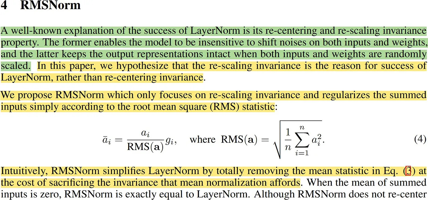
RMSNorm normalizes activation values based on the Root Mean Square of the activation values, as opposed to using traditional Mini Batch or Layer statistics. This has the advantage of scaling activation consistently, regardless of Mini Batch size or Layer. Like other normalization techniques, it also has separate training parameters.
The formula implementation is as follows:
z: Array["B, L or 1, 1"] = (x ** 2).mean(-1, keepdims=True) + self.eps
z: Array["B, L or 1, D"] = x / np.sqrt(z)
return z * self.weight
QKV
The way to calculate QKV is to matmul one weight in GPT and then split it, but Llama have their own weights for QKV, so we need to matmul them separately. Then, for Multi-Head Attention, we reshape each one to separate them by Multi-Head.
# QKV
xq: Array["B, L or 1, D"] = x @ self.q_weight
xk: Array["B, L or 1, D"] = x @ self.k_weight
xv: Array["B, L or 1, D"] = x @ self.v_weight

# ["B, L or 1, D"] -> ["B, L or 1, QHN or KVHN,  HD"]
xq: Array["B, L or 1, QHN,  HD"] = xq.reshape(B, L, self.n_local_heads, self.head_dim)
xk: Array["B, L or 1, KVHN, HD"] = xk.reshape(B, L, self.n_local_kv_heads, self.head_dim)
xv: Array["B, L or 1, KVHN, HD"] = xv.reshape(B, L, self.n_local_kv_heads, self.head_dim)
RoPE #2
Now it’s time to actually apply the RoPE using the values we calculated earlier.
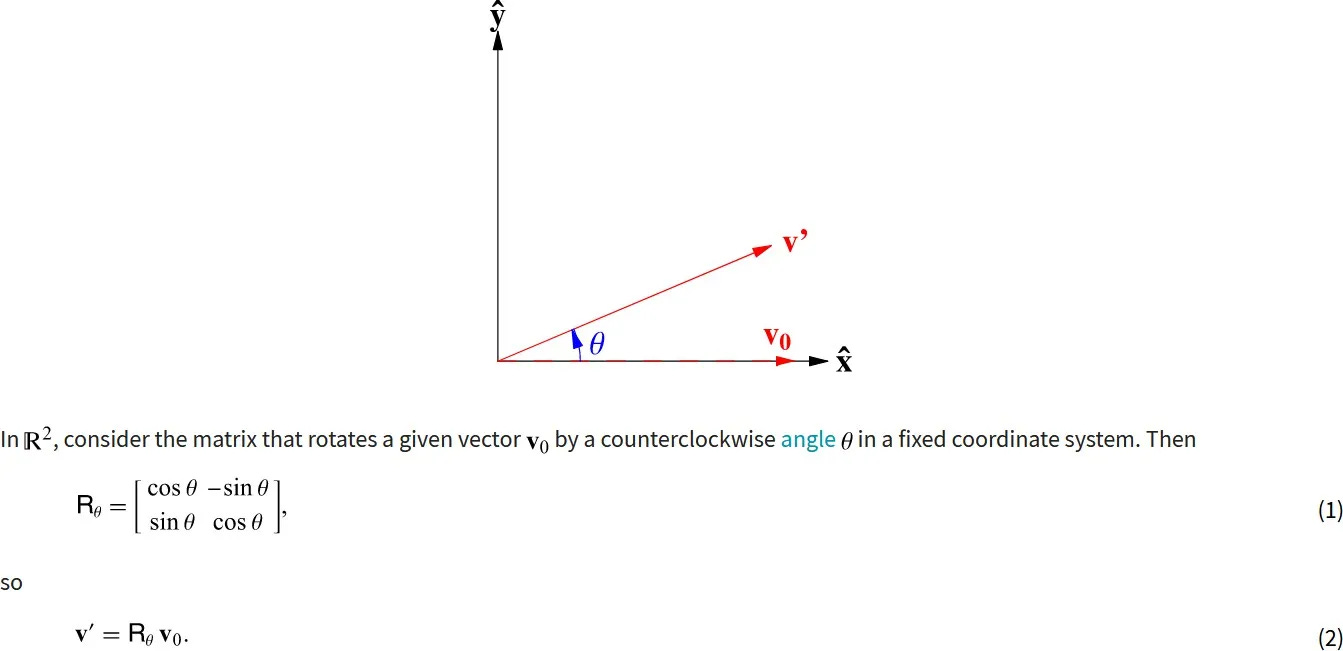
RoPE is a new type of position encoding technique that has the characteristics of both absolute and relative, and performs well because it has the characteristics of both. It only applies to Q and K, dividing each input by the sum of its parts, then multiplying by cos and sin, adding and subtracting the results, and returning the sum back to reshape.
xq_out_r: Array["B, L or 1, QHN,  HD//2"] = xq_r * freqs_cos - xq_i * freqs_sin
xq_out_i: Array["B, L or 1, QHN,  HD//2"] = xq_r * freqs_sin + xq_i * freqs_cos
xk_out_r: Array["B, L or 1, KVHN, HD//2"] = xk_r * freqs_cos - xk_i * freqs_sin
xk_out_i: Array["B, L or 1, KVHN, HD//2"] = xk_r * freqs_sin + xk_i * freqs_cos

xq_out: Array["B, L or 1, QHN,  HD//2, 2"] = np.stack([xq_out_r, xq_out_i], axis=-1)
xk_out: Array["B, L or 1, KVHN, HD//2, 2"] = np.stack([xk_out_r, xk_out_i], axis=-1)
xq_out: Array["B, L or 1, QHN,  HD"] = xq_out.reshape(xq_out.shape[:-2] + (-1,))
xk_out: Array["B, L or 1, KVHN, HD"] = xk_out.reshape(xk_out.shape[:-2] + (-1,))
RoPE are applied after the Q and K have been multiplied by the weights in the attention mechanism, while in the vanilla transformer they’re applied before.
KV Cache
Since the GPT-style generative model is Masked Attention, it is possible to KV Cache. Since the previous result will always be the same, regardless of what comes after it, since we are not allowed to see the next word, we can cache K and V, and Q only needs to compute the last value. The cache is held by max_seq_len(256), so the result of the calculation is put in and then extracted back to the only current length.
# KV Cache
self.cache_k[:B, start_pos: start_pos + L] = xk
self.cache_v[:B, start_pos: start_pos + L] = xv
ks: Array["B, L, KVHN, HD"] = self.cache_k[:B, : start_pos + L]
vs: Array["B, L, KVHN, HD"] = self.cache_v[:B, : start_pos + L]
# (1, 256, 6, 48) -> (1, 5, 6, 48)

# GQA
xk: Array["B, L, HN, HD"] = repeat_kv(ks, self.n_rep)
xv: Array["B, L, HN, HD"] = repeat_kv(vs, self.n_rep)

xq: Array["B, HN, L or 1, HD"] = xq.transpose(0, 2, 1, 3)
xk: Array["B, HN, L, HD"] = xk.transpose(0, 2, 1, 3)
xv: Array["B, HN, L, HD"] = xv.transpose(0, 2, 1, 3)
Here, we fetch the cache values and then transpose them back to reshape them, but this could be done more efficiently by skipping this step. For reference, the maximum size of the KV Cache is 1 × 256 × 6 × 48 × 2 × 6 = 884K on batch size 1. Since it is a 15M model, it takes up about 6% more memory.
GQA(Grouped-Query Attention)
MQA, which is a Multi-query, has the advantage of being compact and memory-saving compared to MHA, which is a Multi-head, but it suffers from poor performance and unstable learning. Therefore, Grouped-query, GQA, was introduced in Llama 2. In Llama 2, GQA was only applied to 70B, but from Llama 3, GQA was applied to all models above 8B. Since we are using a model that was trained without GQA, we do not use GQA, but we have implemented it in the code. We have implemented it by simply copying it by a multiple, and it can be improved by referencing the previous value for future optimization. We have avoided using GQA when n_rep==1.
if n_rep == 1:
    return x
z: Array["B, L, QHN, HD"] = np.repeat(x, n_rep, axis=2)
Scaled Dot-Product Attention
Attentions are calculated separately by Multi-Head.
# Scaled Dot-Product Attention
# ["B, HN, L or 1, HD"] @ ["B, HN, HD, L"] -> ["B, HN, L or 1, L"]
attention: Array["B, HN, L or 1, L"] = xq @ xk.transpose(0, 1, 3, 2) / math.sqrt(self.head_dim)
# `mask` is used only once at the beginning.
if mask is not None:
    attention = attention + mask[None, None, :, :]
attention = softmax(attention)
output: Array["B, HN, L or 1, HD"] = attention @ xv
Masking is only done at the beginning and only the last Q needs to be processed afterward, so no masking is needed. The result can then be obtained with softmax and matmul. Finally, the result of the Multi-Head calculation is reshaped to full dimension to combine the heads and matmul once more.
# ["B, HN, L or 1, HD"] -> ["B, L or 1, D"]
output: Array["B, L or 1, D"] = output.transpose(0, 2, 1, 3).reshape(B, L, -1)
output: Array["B, L or 1, D"] = output @ self.o_weight
Computing the entire QKV at once is only done in the Prefill Phase. At this time, TTFT (Time To First Token) is called Prefill Latency, and only ‘vector @ matrix’ operations need to be performed from the Decode Phase onward. Flash Attention is also effective only when reducing the Prefill Latency during inference, and it performs somewhat well when the input is long.
Feed Forward
In Llama model, Feed Forward uses 3 linear with matmul only and no bias, so unlike GPT, it is not a complete fully-connected layer. We create a swish value from the silu result, multiply it with x_V up-scaled from D to FD, and down-scale it again. Here, the size of FD is FD = 2 * 4 * D / 3, which is D(288), so FD(768).
swish: Array["B, L or 1, FD"] = silu(x @ self.gate_weight)
x_V: Array["B, L or 1, FD"] = x @ self.up_weight
x: Array["B, L or 1, FD"] = swish * x_V
x: Array["B, L or 1, D"] = x @ self.down_weight
SwiGLU
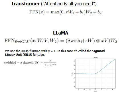
In the paper, the SwiGLU formula looks like this:
Multiplying x_V with swish and matmul it with W_2 is called SwiGLU. This unique combination of multiple feed forwards layers increases the performance of the model. Let x be a real number between approximately −14 ∼ 11, which is the input to the silu function. The silu implementation is as follows:
x * (1 / (1 + np.exp(-x)))Linear
After passing through all the transformer blocks, the final output is only the last logit computed by matmul to speed things up. The transformer block always outputs ["1, D"] as the result after the Prefill Phase.
# ["B, 1, VS"] = ["B, 1(L), D"] @ ["D, VS"]
logit: Array["B, 1, VS"] = h[:, [-1], :] @ self.lm_head_weight
Generation
Now, we generate tokens one after the other using the extracted logit. For simplicity, we’ve omitted sampling from the generation process and only output the Greedy result.
for i, curr_pos in enumerate(range(L, max_new_tokens)):
    if i == 0:  # Prefill Phase
        inputs = input_ids
        pos = 0
    else:       # Decode Phase
        inputs = next_id
        pos = curr_pos
    logits: Array["B, 1, VS"] = self(inputs, pos)
    next_id = logits[:, -1, :].argmax(-1, keepdims=True)
    yield next_id
The first step is Prefill Phase, or sometimes called Summarization. It passes all input and starts at position 0. This is also where Flash Attention comes into play.
From then on, it is the Decode Phase and thanks to the KV Cache, only the last token ID is passed to Q and the result is the also last logit. Here, we omit sampling and only extract the maximum value. If you want to add a sampling process, you can take softmax and implement top_p and top_k.
You can now yield the token ID we generated as a result, decode it in the next step and print the output token to finalize the process.
Example
You can run it like this:
$ python llama3.py "I have a dream"
"""
I have a dream. He dream of a big, beautiful garden full of flower and tree. He dream of playing with hi friend and eating yummy snack.
One day, he wa walking in the garden when he saw

Token count: 50, elapsed: 1.53s, 33 tokens/s
"""
Karpathy has trained the model to a certain extent, and the result is that model is not performing badly. It ran at 33 tokens/s on an M2 MacBook Air.
GitHub
The full source code is available at likejazz/llama3.np.


